The value of TV
Contribution of TV to match outcomes
Now that we have gotten our feet wet with the Champion Ladder data, it’s time to start looking at some actual match results.
We are going to start with Team Value because it’s an interesting mechanic in Blood Bowl that plays a number of complementary roles:
- It provides the initial constraint on team composition, meaning that a fresh team never quite has everything you would like.
- It underpins matchmaking in the Champion Ladder, making TV management an important aspect of long-term strategic decision making.
- It serves as a means of balancing matches by providing inducement cash equal to the difference in TV between the teams.
We will start relatively simply with a few exploratory graphs looking at TV progression within the CCL, before moving on to analysing the effect of TV on match outcomes. Finally, we will take a look at stadium enhancements – one of the unique features of Blood Bowl 2 – and try to figure out if you should bother with them.
In order to easily work with the data on a team-by-team basis, it is first necessary to modify the data from it’s current per-game structure:| Game ID | Home Team Name | Home Team Score | Away Team Name | Away Team Score |
|---|---|---|---|---|
| 1 | XXXX | 2 | YYYY | 1 |
| 2 | AAAA | 0 | BBBB | 3 |
Into something that records data per-team:
| Game ID | Team Name | Team Score |
|---|---|---|
| 1 | XXXX | 2 |
| 1 | YYYY | 1 |
| 2 | AAAA | 0 |
| 2 | BBBB | 3 |
This lets us track the progression of a team, regardless of whether it was playing home or away.
Since the Champion Ladder seasons only run for about six weeks, it is worth looking at just how many games each team ends up playing, since that will affect the options for TV progression we will be looking at.
home_data <- ccl_data %>%
  select(1:10, contains(".0.")) %>%
  set_names(gsub(".*\\.0\\.", "", names(.)))

away_data <- ccl_data %>%
  select(1:10, contains(".1.")) %>%
  set_names(gsub(".*\\.1\\.", "", names(.)))

tv_data_interleaved <- interleave(home_data, away_data)

tv_data_interleaved %>%
  group_by(idteamlisting) %>%
  summarise(n_games = max(row_number())) %>%
  group_by(n_games) %>%
  summarise(n_teams = n()) %>%
  head(5) %>%
  knitr::kable(col.names=c("Total Games", "Number of Teams"), align = "ll")
## Warning: package 'bindrcpp' was built under R version 3.4.4| Total Games | Number of Teams |
|---|---|
| 1 | 24221 |
| 2 | 8466 |
| 3 | 4597 |
| 4 | 2815 |
| 5 | 2096 |
Most teams play very few games in the Champion Ladder. Of the 52,534 total teams that have played across the five seasons, almost half are one hit wonders and 80% have played five or fewer games. At the other end of the scale, there are four teams that have played over 100 games, which is an impressive feat to get through in such a short space of time. If the teams that only play a single game are excluded, the mean number of games per team is 6.75, so once a team gets going it is likely to have a reasonable number of games for us to look at.
TV progression
For the teams that do get going, how does their TV tend to develop? We can explore this question by looking at a heatmap of TV against number of games played by a team. We will break this down by race since the races have different rates of skill and player gain and are therefore likely to have different TV profiles.
tv_data_interleaved %>%
  group_by(idteamlisting) %>%
  mutate(
    team_age = row_number(),
    race = map_chr(idraces, nufflytics::id_to_race)
  ) %>%
  filter(team_age > 1) %>%
  ggplot(aes(x = team_age, y = value)) +
  geom_hex(bins = 45) +
  facet_wrap(~race) +
  viridis::scale_fill_viridis("Count", trans="log10") +
  scale_x_continuous(limits = c(-2, 100),expand = c(0, 2))+ # Cut off at 100 games played for clarity
  scale_y_continuous(limits = c(430, 2350), expand = c(0, 30))+
  labs(title = "TV progression in CCL", subtitle="Team TV against number of games played by team", x = "# Games", y = "TV")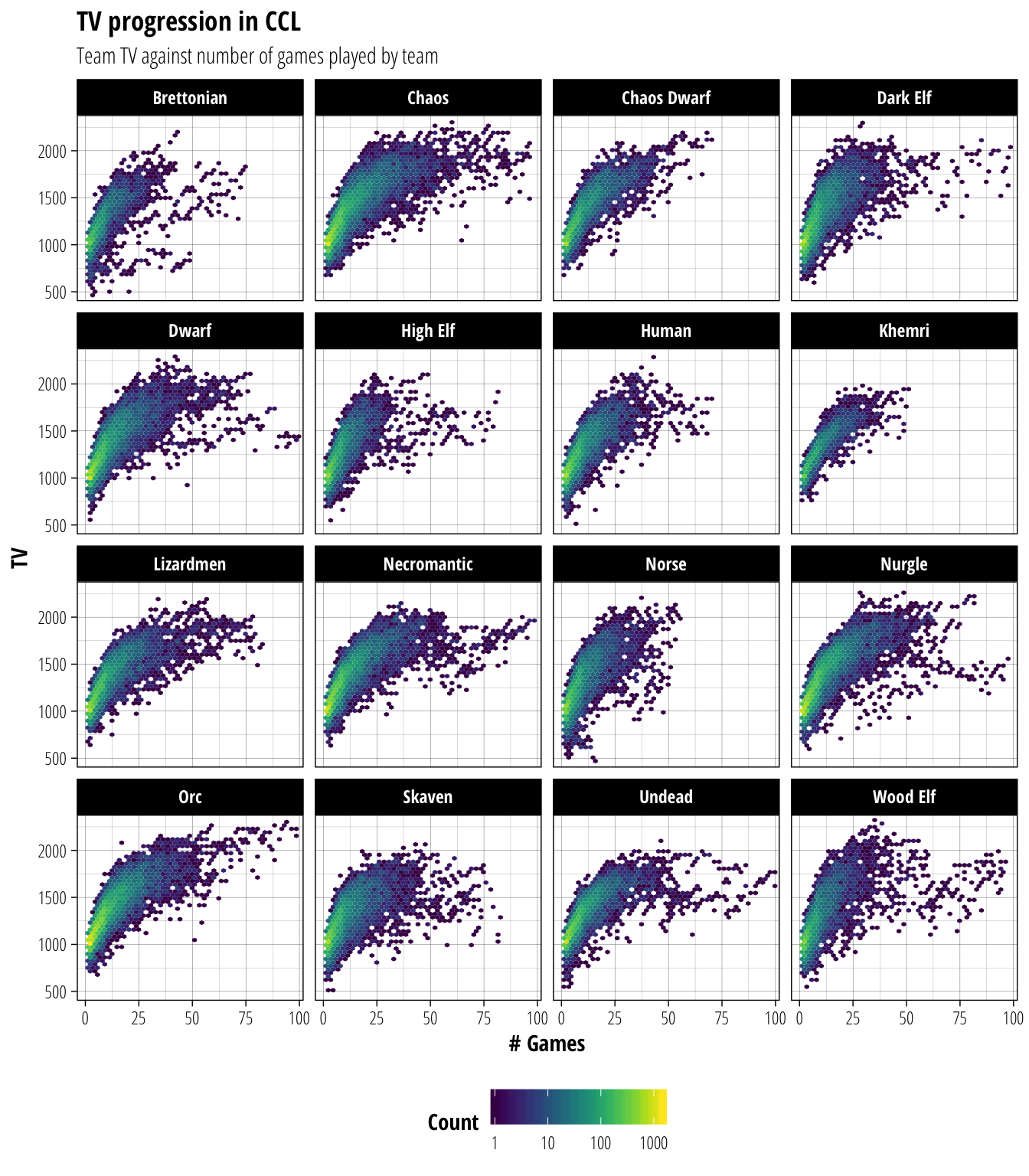
Looking at these heatmaps, the differences between the races are very subtle. Most races reach TV1500 by ~12–15 games, with only small differences between teams that develop quickly (eg. Dark Elf, Wood Elf) and those that develop slowly (eg. Lizardmen, Nurgle). The main difference between races is instead at what point they reach a plateau in TV development. Since so few teams play a large number of games in the Champion Ladder this plateau will be heavily dependent on the specific teams that play that long. However teams that are generally considered powerful at low TV (eg. Undead, Skaven) tend to plateau at a lower TV than teams that just get better the more skills they can take on (eg. Chaos, Orc).
TV Change
Next, we will look at how the TV of a team changes after a match based on it’s starting TV. This may become useful later when we are considering enhancements to our TV-based prediction methods for simulating the results of a league season.
tv_data_interleaved %>%
  group_by(idteamlisting) %>%
  mutate(
    tv_change = lead(value) - value,
    race = map_chr(idraces, nufflytics::id_to_race)
  ) %>%
  filter(!is.na(tv_change)) %>% #remove teams without a second game
  ggplot(aes(x = value, y = tv_change)) +
  geom_hex(bins = 50) +
  viridis::scale_fill_viridis("Count", trans = "log10")  +
  labs(title = "TV gain/loss at different levels", x = "TV", y = "Post match TV change")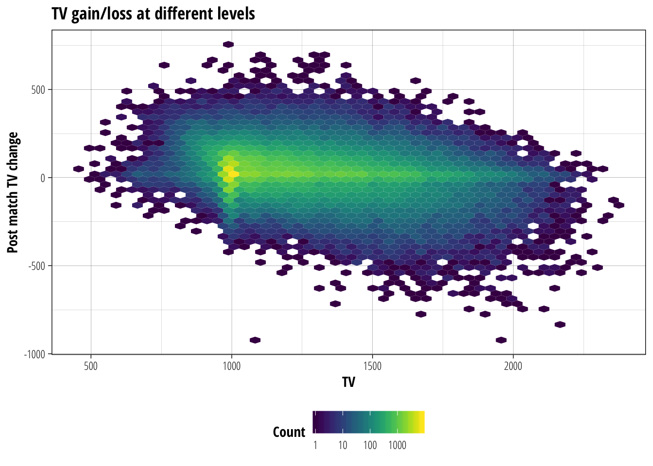
The two most obvious features of this figure are:
- The bright vertical line around TV1000, representing teams playing their first few games.
- The bright horizontal line at a TV change of 0, indicating that most games don’t see a team’s TV change at all
Ignoring these features, there appears to be an inverse linear relationship between TV and TV change. So as the TV of a team increases, you are increasingly likely to suffer a drop in TV after a game. This relationship makes sense because at higher TV most players will have several skills already, making it harder to gain extra skills. At the same time, these high-value players make perfect targets for player removal specialists and their loss can severely impact a team’s TV for the next game.
Matchmaking efficiency
Now that we have some idea of how the TV of a team changes throughout a Champion Ladder season, let’s look at the role of TV as a balancing mechanic by considering the effect of TV difference on game outcomes. The matchmaking algorithm attempts to minimise the TV difference between matched teams, so we should first take a baseline look at how well it manages to achieve that.
# Add game result with 0 = home team loss, 0.5 = tie, 1 = home team win
tv_data <- ccl_data %>%
  mutate(
    tv_diff = teams.0.value - teams.1.value,
    result = with(., case_when(
      teams.0.score >  teams.1.score ~ 1,
      teams.0.score == teams.1.score ~ 0.5,
      teams.0.score <  teams.1.score ~ 0)
    )) %>%
  filter(tv_diff >= -500 & tv_diff <= 500) # A very small number of games have a TV difference larger than 500. I don't know how, but remove them for now.

tv_data %>%
  ggplot(aes(x = tv_diff)) +
  geom_histogram(binwidth = 10) +
  scale_x_continuous("Home team TV difference", breaks = seq(-500, 500, by = 100), minor_breaks = NULL) +
  labs(title = "Champion Ladder Matchmaking Effectiveness", y = "# Games")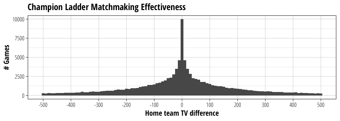
The median outcome is obviously to have a perfectly matched game, with just under 10,000 games out of the 107,556 games in total. 50% of the matches fall within \(\pm\) 90TV, so without spending treasury cash most games will have no more than a Bloodweiser Babe as inducements. The majority of games (90%) fall between \(\pm\) 350 TV, which seems pretty reasonable considering how many Champion Ladder games get played in a day. Although ending up in that 5% tail of being down 500–350 TV is never a fun situation.
Effect of TV difference on game result
If TV-based inducements were a perfect balancing mechanic, we would see a 50% win rate regardless of the TV difference between two teams. There are obvious reasons why we do not expect it to be perfect, but how well do inducements make a fair match between mismatched teams?
Since it is reasonable to assume that concessions are more likely to occur in a heavily uneven matchup, we will look at game results as a function of TV difference both including and excluding games that resulted in concessions.
tv_data_noconceeds <- tv_data %>%
  filter(teams.0.mvp == 1) # Remove conceded games

tv_plot <- function(data) {
  ggplot(data,aes(x = tv_diff)) +
    geom_histogram(aes(fill = factor(result)),binwidth = 10, position="fill", alpha = 0.7) +
    geom_smooth(aes(y = result), colour = "black", se = F, method = "glm", method.args = list(family = "binomial")) +
    scale_fill_manual("Result", values = c("#d73027", "#ffffbf", "#4575b4"), label = c("Away win", "Tie", "Home Win")) +
    scale_y_continuous("Proportion", breaks = seq(0, 1, by = 0.1), labels = function(b) {paste0(as.numeric(b)*100, "%")}, expand = c(0, 0))+
    scale_x_continuous("Home team TV difference",breaks = seq(-500, 500, by = 100), expand = c(0, 0))+
    ggtitle("Win probability by TV differential")
}
p1 <- tv_plot(tv_data) + labs(subtitle = "All games")
p2 <- tv_plot(tv_data_noconceeds) + labs(subtitle = "Completed games")

cowplot::plot_grid(p1,p2)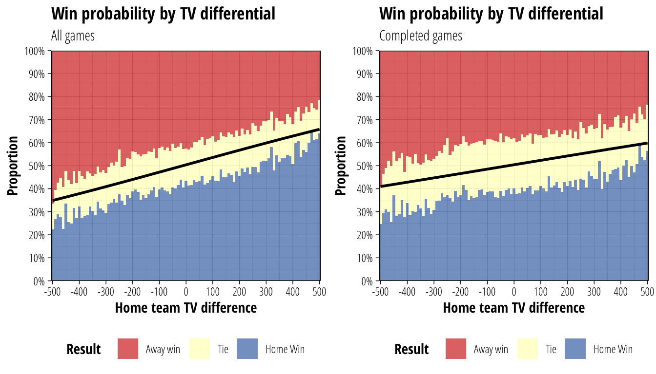
The coloured bars above show the observed frequency of game results with different TV differences. For example, looking at completed games only, an even match sees about 40% of games won by the home team, about 40% won by the away team and about 20% of games ending in a tie. If instead you look at games where the home team has a +400 TV advantage, about 50% of games are won by the home team, 30% by the away team and 20% are tied.
The black line shows the outcome of fitting a logistic regression to the data, which models log(\(\frac{\textit{prob. home win}}{\textit{prob. away win}}\)) as a function of TV difference. This regression indicates the expected value for the home team of the match where a win is worth 1 point, a tie \(\frac{1}{2}\) and a loss 0. This can effectively be thought of as the win probability of the home team if tied outcomes are ignored. The fact that the line on the right is much flatter than the left suggests our assumption about concessions being more likely in unbalanced matches is correct, so we will only consider completed games for the rest of the analysis.
What the right hand figure tells us is that inducements provide a reasonably good balancing mechanic. Differences in TV provide only marginal changes to win probability; even at the extremes a team with +500 TV will only win about 60% of games that aren’t tied.
Stadium enhancements
Stadium enhancements are an interesting addition to the game, costing $100K (plus $100K upgrading the stadium to level 2) but not adding to a team’s TV. I assume the argument for why this is the case is that enhancements provide their benefit equally to each team, so shouldn’t affect the TV of the purchasing team. However, it’s pretty easy to imagine situations where one team gets much more value out of the enhancement than their opponent (Deathroller Dwarves with a free bribe, anyone?), and teams can be built to take advantage of having their home ground enhancement in ~50% of games they play. It is therefore worth considering what the true value of stadium enhancements are and if they make a difference to a team’s win rate.
Before answering that question, we should summarise what stadium enhancements are used by Champion Ladder teams to understand more specifically what we are measuring.
tv_data_noconceeds %>%
  filter(!is.na(structstadium)) %>%
  group_by(structstadium) %>%
  summarise(total = n()) %>%
  arrange(desc(total)) %>%
knitr::kable(col.names = c("Stadium Enhancement", "# Matches"), align = "ll")| Stadium Enhancement | # Matches |
|---|---|
| SecurityArea | 1586 |
| RefreshmentArea | 1303 |
| RefereeArea | 1147 |
| Roof | 1108 |
| FoodArea | 1030 |
| Astrogranit | 927 |
| Nuffle | 520 |
| Bazar | 377 |
| ElfTurf | 341 |
| VIPArea | 150 |
Of the 80,481 completed games in the dataset, only 8,489 (10.5%) have a stadium enhancement. This makes it a reasonably small sample size, but it should be large enough to detect any major effects on win rate. Most of the possible enhancements are well represented in the dataset, meaning that our results should apply to stadium enhancements more generally, rather than just to one or two popular ones.
Because I understand things much better when there are pretty pictures let’s try a quick visual check to see if there is likely to be an effect we can detect. Taking the plot above, we will overlay a logistic regression fitted only with data from games containing a stadium enhancement in green.
p2 + geom_smooth(
  data = function(d) filter(d,!is.na(structstadium)),
  aes(y = result),
  se = F,
  colour = "#4daf4a",
  method = "glm",
  method.args = list(family = "binomial")
  )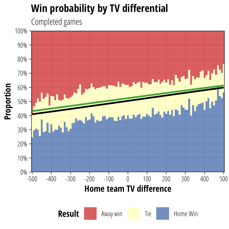
This crude approach does suggest that a stadium enhancement has an effect on win rates. Since the green line sits above the black line calculated from all games, stadium enhancements are associated with a slight increase in the home team’s chance of winning the game.
We can assess this more formally by fitting a logistic regression with both presence of a stadium enhancement and TV difference as independant variables.
model = glm(result ~ tv_diff + !is.na(structstadium), data = tv_data_noconceeds, family = "binomial")

summary(model)
##
## Call:
## glm(formula = result ~ tv_diff + (!is.na(structstadium)), family = "binomial",
## data = tv_data_noconceeds)
##
## Deviance Residuals:
## Min 1Q Median 3Q Max
## -1.37941 -1.16521 -0.00413 1.15510 1.33462
##
## Coefficients:
## Estimate Std. Error z value Pr(>|z|)
## (Intercept) 8.262e-03 7.483e-03 1.104 0.269536
## tv_diff 7.411e-04 3.775e-05 19.629 < 2e-16 ***
## !is.na(structstadium)TRUE 8.449e-02 2.343e-02 3.606 0.000311 ***
## ---
## Signif. codes: 0 '***' 0.001 '**' 0.01 '*' 0.05 '.' 0.1 ' ' 1
##
## (Dispersion parameter for binomial family taken to be 1)
##
## Null deviance: 86584 on 80480 degrees of freedom
## Residual deviance: 86146 on 80478 degrees of freedom
## AIC: 111443
##
## Number of Fisher Scoring iterations: 3The relevant parts of the regression summary can be found after the Coefficients: heading. Both the tv_diff and !is.na(structstadium)TRUE coefficients are statistically significant (p < 0.001), suggesting that TV difference and the presence of a stadium enhancement both contribute to the home team’s probability of winning.
The best way to explain what those coefficients mean for win probabilities is to show an example of the change in probabilities as either of the factors change. Since this is a logistic, rather than a linear regression, the precise contributions will be different at different points along the TV difference scale, however in our situation these differences are minimal and so a single example will be sufficient to show the relationship.
Starting from a situation of perfectly matched teams with no stadium enhancement, the predicted home team win probability is 50.2% (95% CI 49.8–50.5%). In other words, a perfectly balanced match. Increasing the home team’s TV to be 100 more than the opponent produces a predicted win rate of 52.1%, an increase of 1.9 percentage points (95% CI 1.6–2.0 percentage points). If we instead keep the teams with equal TV, but add a stadium enhancement, the predicted win rate is now 52.3%, an increase of 2.1 percentage points (95% CI 0.96–3.3 percentage points).
The closeness of these estimates of a 1.9 and 2.1 percentage point increases in win rate means our best guess is that a stadium enhancement is roughly equivalent to having an additional 100TV on the team (strictly speaking, it’s equal to having an additional 113.5TV, but 100TV is close enough). The confidence interval for the stadium enhancement effect is quite large however, due to the sample size issues described above. Converting that interval into TV equivalents suggests an value for stadium enhancements somewhere between 60–180TV
Stadium enhancement effects
Getting more data from future seasons will help to narrow down the size of this effect, however to summarise the main conclusions from above:
- Stadium enhancements provide a moderate advantage to home teams
- This advantage is roughly equivalent to an additional 60–180TV
- Our best guess of this advantage (~113TV) suggests that enhancements are fairly priced at 100K
- To have a truly neutral effect on game outcomes, they should add to the TV of the purchasing team
Share this post
Twitter
Google+
Facebook
Reddit
LinkedIn
StumbleUpon
Email